Grounded World Models: Efficient and Verifiable Structural Causal Prediction 2 The Grounded World Model, Formally 4 Discussion

3 Benchmarking the Costs of Grounded Prediction

3.1 Task and protocol

We benchmark Primordia’s v1 investment GWM against a reference NWM based on a state-of-the-art LLM as of June 2026 (Claude Opus 4.8), on the domain of fundamentals-based public equity analysis.¹⁰¹⁰10Compare (Vals AI, 2026). As illustrated there, performance is nearly equivalent across frontier models of various sizes and families, which licenses our choice to focus on a single representative LLM for comparison. The unit of measurement is a single case: an analysis of a single traded stock at a given point in time. The task: given a fixed evidence set about one company, and optionally a set of assumptions and counterfactual interventions, predict its 12-month forward return as a predictive distribution and emit an investment recommendation. The inputs, identical across arms, are (i) a research dossier—a body of qualitative and quantitative findings assembled from public sources by web research—and (ii) structured fundamentals—the company’s reported financials. The required output is a predictive distribution (PD) over the 12-month forward return; the GWM produces a set of samples from the joint distribution over present and future latent covariates, future fundamentals, and forward price, while NWM produces a five-scenario table (a probability and an implied price per scenario), a probability-weighted target price, an expected return, a directional recommendation (LONG or “buy”, SHORT or “sell”, HOLD or “neutral”) with a conviction, accompanied by a full investment memorandum following a standard fundamental analysis framework that is compatible with our GWM’s construction logic. For comparability, we summarize the GWM’s output in the same format as the NWM.¹¹¹¹11The GWM’s directional recommendation and conviction are deterministic functions of the PD, following industry-standard decision rules. Typically, the decision support workflow for an investment decision (see 4.1) requires a stream of counterfactual queries and therefore of PD generation tasks: canonically, the first generated PD serves as a baseline, while subsequent PDs are generated with different sets of assumptions and counterfactual interventions.¹²¹²12For instance, a typical analyst query like “what would it take for this to be a LONG instead of a HOLD” might require a decision support system to make dozens of queries to find plausible combinations of assumptions generating the required results. The sample comprises 20 cases drawn at random from the deployed universe; the comparison is per-case and the reported figures are medians over the sample.

Both arms receive the same inputs and must emit the same output schema; they differ only in whether these quantities are read from a grounded posterior (the GWM; Eq. (1)) or asserted directly by a language model. The narrative-WM (NWM) arm is the latter: an ablation that removes the posterior and requires the model to assert the scenario set, its probabilities, the target price, the expected return, and the recommendation itself. Explanation quality is scored over 20 one-shot NWM memos, by a tool-backed judge (estimation methodology in Appendix C). Figure 2 shows the protocol; a fully worked single case is given in Appendix E.

Reproducibility.

The research dossiers and structured fundamentals are assembled entirely from public sources. The NWM harness, the explanation-quality judge agent (Appendix C), the reference GWM outputs, and a battery of GWM predictive distributions under counterfactual interventions are released as a self-contained public benchmark¹³¹³13https://github.com/primordia-ai/gwm-nwm-comparison-public; the per-case input artifacts are available on request. The GWM side is also reproducible directly, on the free tier at https://app.primordia.ai.

Figure 2: The benchmark task. A case is one stock at a point in time; the target

Y

is its 12-month forward return, served as a stream of queries that share one model and vary the assumptions

u

and/or interventions

\mathrm{do}(a)

(a baseline

u_{0}

, then re-forecasts and what-ifs). Both arms take identical inputs, follow a shared analysis framework, and report in a common schema; they differ only in the middle—the GWM is built once, then answers each query by

O(1)

inference at flat cost

c_{\mathrm{PD}}

, while the NWM re-runs per query at a cost rising with the XQ bar (Eq. (8)). A tool-backed judge scores both on

(S,\mathrm{CC},\mathrm{HtV},R)

; cumulative cost and break-even

Q^{\star}

are in Figure 4.

3.2 Benchmark results: efficiency and explanation quality

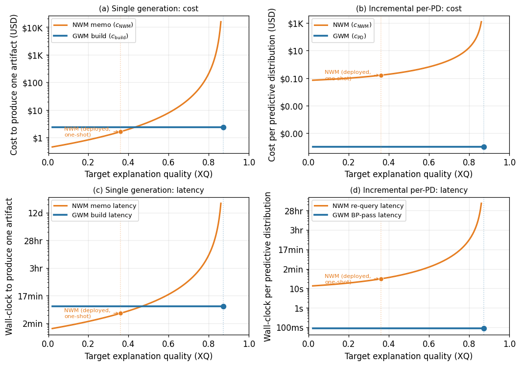
We benchmark the two arms on efficiency and explanation quality, then combine them. Both arms’ efficiency scales with underlying model size, but two things separate them (Figures 3, 4): the GWM’s model is far smaller, and—decisively—a GWM posterior is exact given its evidence, so it delivers its maximal explanation quality (the conditioning-limited ceiling $A_{\mathrm{GWM}}$ ) at every predictive distribution regardless of budget and latency constraints, whereas raising a NWM’s XQ demands more thinking tokens, tool calls, and validator iterations, driving cost and latency super-linearly toward an attainability ceiling $A_{\mathrm{NWM}}$ it can only approach.¹⁴¹⁴14This shared label $A_{\mathrm{NWM}}=A_{\mathrm{GWM}}$ is a deliberately generous convention, not a claim that spending enough tokens actually closes the gap to the GWM. Proposition 5 shows the narrative arm’s true structural ceiling on the three mechanism-checked axes ( $S,\mathrm{CC},\mathrm{HtV}$ ) is strictly below the GWM’s at every budget: in the weather-forecasting illustration of Section 2.7 and 2.6, no amount of narration lets an LLM’s forecast satisfy the do-calculus identities that a numerical model enforces by construction, so more tokens raise the attained XQ along the cost curve of Eq. (8) without ever closing that structural gap. We cannot establish how much lower the true ceiling is, nor do we have enough data to fit the blow-up exponent $\eta$ well enough to extrapolate the cost curve out to it empirically (Appendix C); we therefore take the best case for the NWM—its ceiling generously equated to the GWM’s—so that every divergence and dominance result we report (Corollary 1) is conservative, holding a fortiori against the true, lower ceiling. We score quality on the bounded attainability $A=\prod_{i}c_{i}=\exp(\mathrm{XQ})\in(0,1]$ of Eq. (7) and price both arms on two consistent bases—single-generation and incremental per-PD—via the NWM per-PD cost model of Eq. (8) and the break-even of Eq. (12). Appendix C formalizes the two levels a NWM faces—a structural ceiling no budget can clear (Proposition 5, which we generously equate to the GWM’s) and the lower level it attains under finite compute (Proposition 6)—and proves that, because XQ aggregates multiplicatively, the GWM dominates at every finite budget (Corollary 1).

Per-case generation cost and latency.

A Primordia v1 case costs $c_{\mathrm{build}}=\$2.35{}$ ( $\approx\!408{}$ s). The NWM arm (Opus 4.8) costs a measured $c_{\mathrm{NWM}}=\$1.63{}$ ( $\approx\!230{}$ s) for a standard sourced memo—the median over 20 cases (range $1.21–$1.82)¹⁵¹⁵15Measured via a custom LLM agent given the same knowledge base (research dossier, structured fundamentals) used to build the v1 GWM, instructed to form every scenario, probability, target price, and recommendation itself; cost is cache-adjusted API spend over the full agentic tool loop (June 2026 pricing). At this single-generation budget the GWM build costs and takes more than one NWM memo ( $\$2.35{}$ vs $\$1.63{}$ ; $1.8\times$ the latency)—not a contradiction, since the build is a one-time flat cost and the NWM’s own cost/latency rises with the XQ target, crossing above the GWM’s past $A\approx 0.43$ (Section 3.2)., and $3c_{\mathrm{NWM}}$ for a full evidence-chain artifact.

Explanation quality of the two arms.

The arms separate on all four XQ axes. The GWM is exact-by-construction on the mechanism ( $S=\mathrm{CC}=1$ ), with $\mathrm{HtV}=0.92$ and $R=0.95$ . The narrative arm’s measured components are all well below $1$ ( $S=0.83$ , $\mathrm{CC}=0.88$ , $\mathrm{HtV}=0.67$ , $R=0.73$ ; Table 4)¹⁶¹⁶16Attainments at the deployed budget, not ceilings, each measured conservatively: CC is the two-step $\min(\mathrm{CC}_{\mathrm{stat}},\mathrm{CC}_{\mathrm{int}})$ estimator of Appendix C (the static step binds at the deployed budget); $R$ is the simplex-volume residual control of Definition 11, granted only as the NWM’s generous ceiling.. Because XQ aggregates multiplicatively, these place the NWM’s deployed joint correctness at $\prod_{i}c_{i}=0.36$ against the GWM’s $0.87$ —a $2.4\times$ gap at equal (deployed) cost; a product is capped by its weakest factor. Appendix E reports the same scorecard for the worked case (Table 3).

Cost and latency to reach a quality target.

Pricing both arms on two consistent bases (Figure 3) makes the divergence concrete in dollars and wall-clock. Single generation: a single NWM memo undercuts the GWM build’s cost at a low bar but crosses it at $A\approx 0.43$ as the output blow-up takes over. Incremental per-PD: the GWM answers each PD at a flat $c_{\mathrm{PD}}=\$1.0\times 10^{-6}{}$ in $0.086$ s, while the NWM’s cost and latency climb without bound toward the ceiling— $357\times$ slower on a measured warm re-query ( $30.9$ s) today, and the gap widens as the bar rises.¹⁷¹⁷17Latency follows the identical divergence shape as cost (the same output-token blow-up drives both), rescaled by the measured seconds-per-dollar ratio at the deployed attainment rather than a separate token-rate model (Appendix I). The conditioning-limited ceiling itself falls with forecast horizon, but that horizon binds both arms equally. By Proposition 1 this is a statement about prediction quality, not merely its proxy.

Refer to caption — Figure 3: Cost (top) and latency (bottom) to reach a target explanation quality, on two consistent bases. (a)/(c) Single generation: the GWM’s one-time build vs. the NWM’s full sourced memo, each anchored at its measured cost/latency at the deployed attainment. (b)/(d) Incremental per-PD: the GWM’s flat belief-propagation pass vs. the caching-aware NWM re-run of Eq. (8) and its latency analogue. The GWM is flat and sits at the ceiling in every panel; the NWM diverges toward the same (generously shared) ceiling $A_{\mathrm{GWM}}$ (dotted), with the deployed one-shot NWM marked ( $A\approx 0.36$ ). Target axis: bounded attainment $A=\exp(\mathrm{XQ})\in(0,1]$ (Eq. (7)). Log $y$ -axes; values from Appendix I.

Amortizing the build.

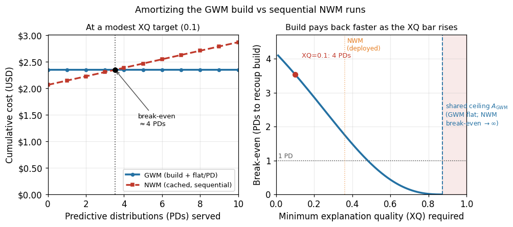
The single-generation parity is an artifact of $Q=1$ . The GWM pays $c_{\mathrm{build}}$ once, then answers every PD at a flat $c_{\mathrm{PD}}=\$1.0\times 10^{-6}{}$ in $0.086$ s; the NWM re-runs per PD, even granted its own best-case caching amortization. The break-even $Q^{\star}(\mathrm{XQ})$ of Eq. (12) (Figure 4) shows the build recouped after $\approx\!4{}$ PDs at a modest target ( $0.1{}$ ), collapsing to a single PD as the bar rises; above the NWM ceiling ( $\approx\!0.87{}$ ) no number of runs reaches the target. The same logic applies to wall-clock: the GWM’s slower build is repaid almost immediately once queries stream, since every follow-on PD answers $357\times$ faster than a warm NWM re-query.¹⁸¹⁸18 $1.8\times$ slower than one NWM memo on the single-generation basis (Section 3.2). Appendix E works one real (anonymized) case end-to-end across the PD stream.

3.3 Limitations

Our empirical evidence is deliberately scoped, and we are explicit about what is measured versus assumed. The strongest results are direct measurements over the deployed system: per-case build cost ( $c_{\mathrm{build}}=\$2.35{}$ /case over 1,184 cases from production logs, $\approx\!408$ s of wall-clock), the GWM’s flat per-PD inference cost and latency ( $c_{\mathrm{PD}}\approx\$1.0\times 10^{-6}{}$ /PD, $0.086$ s/PD), and the narrative arm’s per-case generation cost and latency ( $c_{\mathrm{NWM}}=\$1.63{}$ , range $1.21–$1.82; $\approx\!230$ s) and warm re-query latency ( $30.9$ s, the same measured calls that anchor the incremental-PD cost curve). All come from a single domain—equity investing—so the magnitudes should be read as evidence that the architectural gap is real and large, not as a cross-domain performance benchmark; a live track record is out of scope here by design.

The explanation-quality comparison is likewise measured by proxy. We score the narrative arm’s structural components ( $S$ , $\mathrm{CC}$ , $\mathrm{HtV}$ ) with a tool-backed judge over 20 cases (Section 3.2). The GWM’s own ceiling and its residual-control values $R$ are by-construction (exact posteriors given evidence), not independently audited, and the cost–XQ blow-up exponent is an empirically justified modeling assumption rather than a fit. The XQ $\to$ PQ proxy (Proposition 1) rests on Assumptions 1–2, plausible but unverified for any specific domain.

Finally, one bound is not an artifact of measurement at all: even a perfectly specified, perfectly conditioned GWM is capped by the system’s intrinsic predictability horizon (Section 2.7), which limits the residual-control component $R$ at long lead times. This is a property of the world, not the model, and it bounds both architectures equally.